NLP · Distillation · 2024

On polarity, distillation,
and the cost of compute.

Abstract: Binary sentiment classification on the Amazon Polarity corpus, run as a ladder: a random classifier, a TF-IDF logistic regression, a fine-tuned DistilBERT, and finally a TinyBERT student distilled from the best of them. The question underneath is not how accurate we can get, but how little we can spend: how few labels, and how small a model, still arrive at the same place.
Data: Amazon Polarity, 4 M reviews, balanced positive / negative. We worked on a 10% sample: 306 k train, 54 k validation, 40 k test. Negative reviews run slightly longer than positive ones, 94 words against 88.
Method: TF-IDF baseline → DistilBERT fine-tuning → augmentation study (synonym, zero-shot, GPT-2) → training-fraction sweep → distillation into TinyBERT.

The baseline is closer than you would think

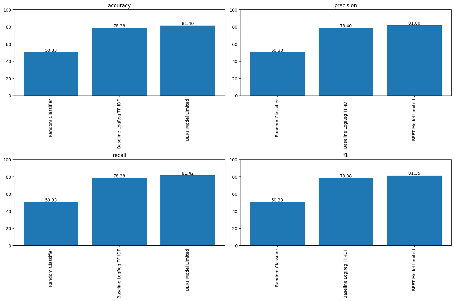
A random classifier lands at 50.33%. The corpus is balanced, so that is the floor. A TF-IDF logistic regression, fit on 30 k reviews after lowercasing, stopword removal and Porter stemming, reaches 78.38%. That is the number worth holding on to: three quarters of the task is available for the price of a sparse matrix and a convex solver.

Accuracy, precision, recall and F1 for the random classifier, the TF-IDF baseline and a compute-limited DistilBERT — Fig. 1 · Random, TF-IDF logistic regression, and a DistilBERT fine-tuned on 32 labelled examples.

The transformer, and its appetite

We fine-tune distilbert-base-uncased: 66.4 M trainable parameters, sequences capped at 128 tokens (reviews average about 90 and top out at 272), and the [CLS] hidden state passed through dropout into a single sigmoid unit. Adam, binary cross-entropy, a conservative learning rate, and the backbone left trainable, which turns out to matter more than anything else we varied.

Fine-tuned on 32 labelled examples, it reaches 81.40%. Better than the baseline, but only just, and on a sample that small the seed does much of the talking.

Student-teacher knowledge distillation diagram — Fig. 2 · Bert-3PO lurking in Amazon's offices.

Can augmentation buy labels?

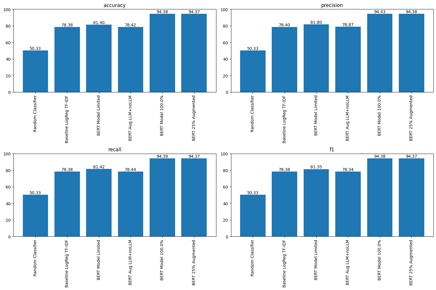
Partly, and only while the synthetic text stays plausible. Substituting WordNet synonyms with nlpaug, five variants per review, takes the 32-label model from 81.40% to 85.24%. Generating fresh reviews with GPT-2 helps less. Pushing that augmentation to 20× collapses the model to 78.42%, below the version we were trying to improve, because the generator writes unconvincing negative reviews, and duplicated noise is still noise.

A zero-shot LLM classifier scores 93.10% having seen none of our labels, which we read with suspicion rather than pride: a model pre-trained on the open internet has almost certainly met this task, or something close enough to it, already.

How much data does it actually need?

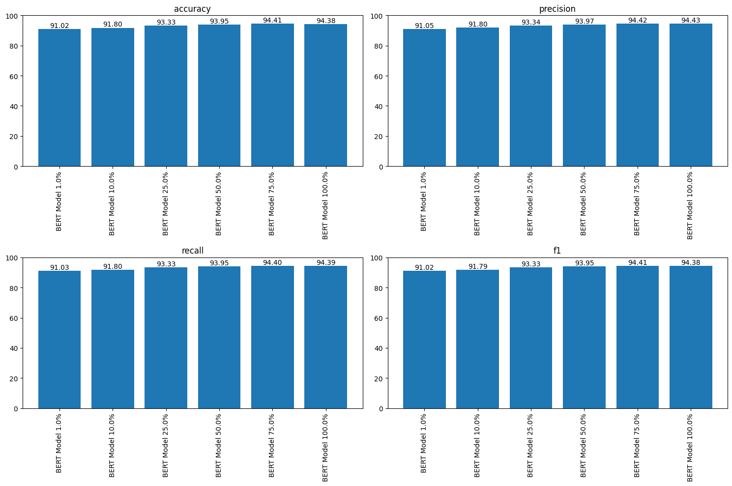
Fine-tuning on 1, 10, 25, 50, 75 and 100% of the training set (one epoch each), the curve flattens almost immediately. One per cent of the data already gives 91.02%; a quarter gives 93.33%; everything gives 94.38%, and the model trained on three quarters (94.41%) is indistinguishable from it.

Accuracy, precision, recall and F1 for DistilBERT trained on 1% through 100% of the data — Fig. 3 · Returns flatten fast. The last three quarters of the corpus buy about one point.

The two findings meet in the middle. Synonym-augmenting a quarter of the training set until it is the size of half of it yields 94.37%: the full-data number, from a quarter of the real labels.

All models compared: random, TF-IDF, limited DistilBERT, over-augmented DistilBERT, full-data DistilBERT and 25% augmented — Fig. 4 · Every model side by side. Note the over-augmented run, fourth from the left, sitting below the baseline it was meant to beat.

Distillation

The full-data DistilBERT becomes the teacher; the student is TinyBERT (prajjwal1/bert-tiny: two layers, hidden size 128, two attention heads, against DistilBERT's six, 768 and twelve). The student trains on a weighted sum of two losses: ordinary cross-entropy against the true labels, and the divergence between its own temperature-softened predictions and the teacher's.

teacher_logits = self.teacher_model(x, training=False)

with tf.GradientTape() as tape:
    student_logits = self.student_model(x, training=True)

    task_loss = self.task_loss_fn(y_true, student_logits)

    teacher_probs = tf.nn.softmax(teacher_logits / self.temperature, axis=-1)
    student_probs = tf.nn.softmax(student_logits / self.temperature, axis=-1)
    distillation_loss = self.distillation_loss_fn(teacher_probs, student_probs)

    total_loss = (self.alpha * task_loss) + ((1 - self.alpha) * distillation_loss)

The student carries 4.39 M parameters against the teacher's 66.4 M (16.7 MB on disk against 253 MB), and trains roughly three times faster per epoch. It scores about 90% across accuracy, precision, recall and F1, against the teacher's 94%.

Lessons

Four points of accuracy is what a fifteen-fold reduction in size cost us here, and whether that is a bargain depends entirely on where the model has to run. The augmentation results cut the same way: synthetic data substitutes for labels only while it remains convincing, and the moment it stops being convincing is visible in the metrics long before it is visible in the text.